Lab: Phasor: Passive RL Circuit(May 11, 2017)

Date: May 11, 2017

Phasors: Passive RL Circuit Response

 This is basic understanding of phasors. On the board, we derived how to look at phasors.

This was an activity to determine the difference between two phasors.

 These are all the different forms in which a phasor could be existent.

 On the left, we see all the rules for phasor calculation. On the right are all the examples of phasor calculations.

 In this example, we solved a phasor equation, then reconverted it to a time-dependent voltage. The magnitude of the voltage goes in front of the cosine function. The phase angle goes inside the cosine function, after the time.

 In these examples, we add together two voltages by solving them in the phasor domain and converting them to the time-dependent domain. We take the answer and solve for current in time-dependent domain.

 This is the pre-lab in which we find the frequency, the gain, and the cutoff using the phasor domain we just learned.

 This was the first frequency found at 70K hz.

This was the built circuit for phasors. 

Lab: RLC Circuit Response (May 9, 2017)

Date: 05/09/2017

RLC Circuit Response

 This is a schmitt trigger. We learned about it in class. It is a comparator circuit with hysteresis implemented by applying positive feedback to the noninverting input of a comparator or differential amplifier. It is an active circuit which converts an analog input signal to a digital output signal.

 We continue to analyze step response in series RLC circuit in this example. Once again we find alpha and omega and use that to find the voltage as a function of time.

  We continue to analyze step response in series RLC circuit in this example. Again, we find alpha and omega and use that to find the voltage as a function of time.

This is the pre-lab for RLC circuit response.

This is the built circuit.

 This is further analysis of RLC circuits.

These are the output graphs on four step response. 

Lab: Series RLC Circuit Step Response (May 02,2017)

Date: 05/02/2017

Series RLC Circuit Step Response

 This is our introduction to phase response. On the left side, we find the initial values of current and voltage. Then we have to find the derivative of current and voltage. Finally we found the current and voltage after an infinite amount of time.

 This is derivation to determine the characteristics of any given step response RLC circuit.

 We are analyzing a source free RLC. In order to analyze the circuit, we have to find alpha and omega. In this case, it's over damped. There are three types that the circuit would be: over damp, critically damped, or underdamped.

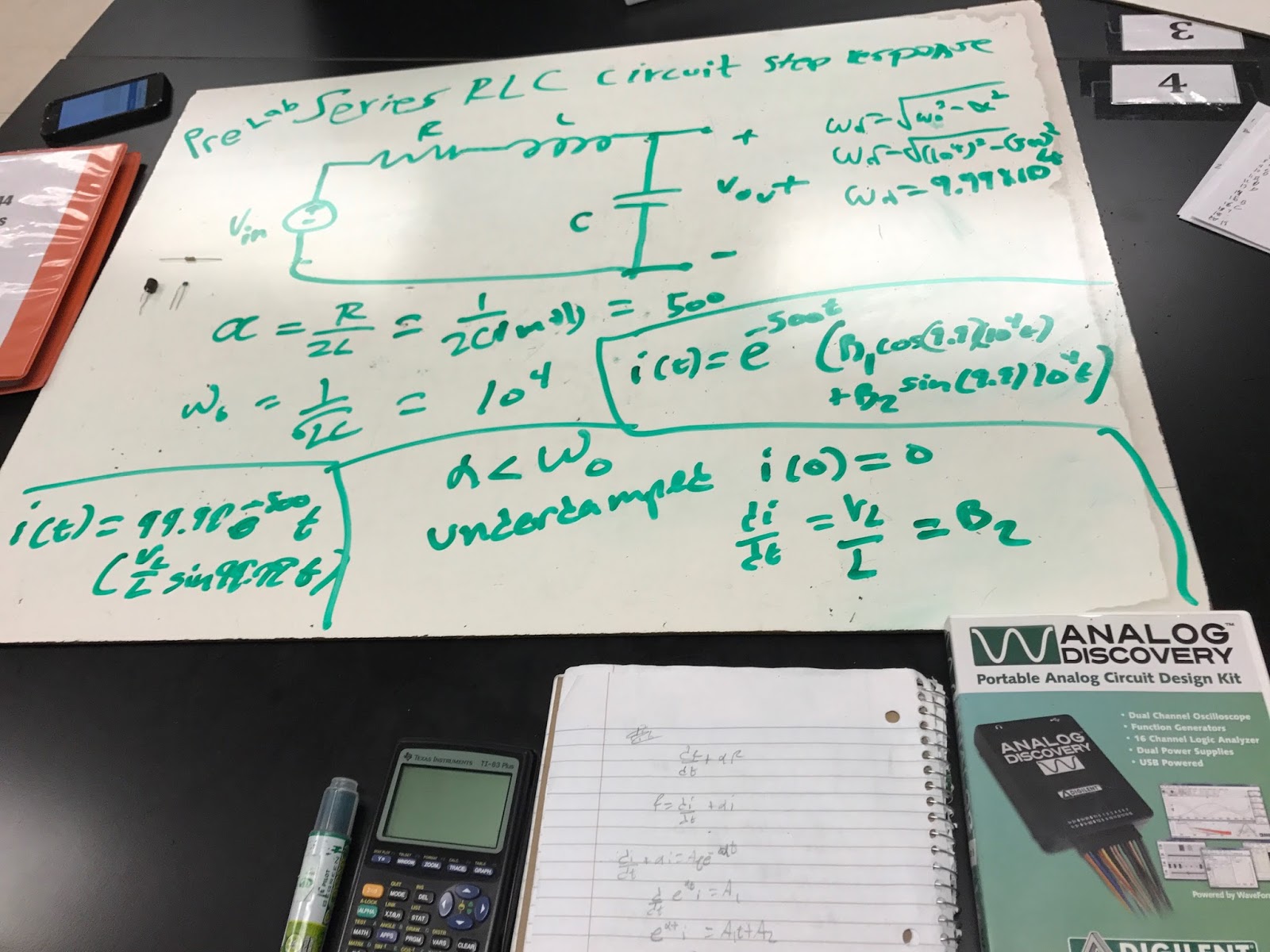
 This is the pre-lab for the rLC step response. We determined the alpha and omega which helped us determine that the circuit is underdamped. The we solved for the current as a function of time.

  This is more information added.

We solved for alpha and omega for a parallel RLC step response. In a parallel step response, we find the voltage as a function of time instead of the current. 

Lab: Superposition (March 23, 2017)

Date: 3/23/2017

Superposition

 In these photos, our group looked at linearity property. Linearity property simply states that we can use matrix analysis, otherwise known as linear algebra to solve circuits. We are also using KVL to analyze the circuit.

 In this example, we are analyzing superposition. Superposition principle states that the voltage across or current thought an element in a linear circuit is the algebraic sum of the voltages across that element due to each independent source acting alone. We make the voltage source open circuit. The solved using loops.

 This is another example of super position in which we find the equivalent resistance.

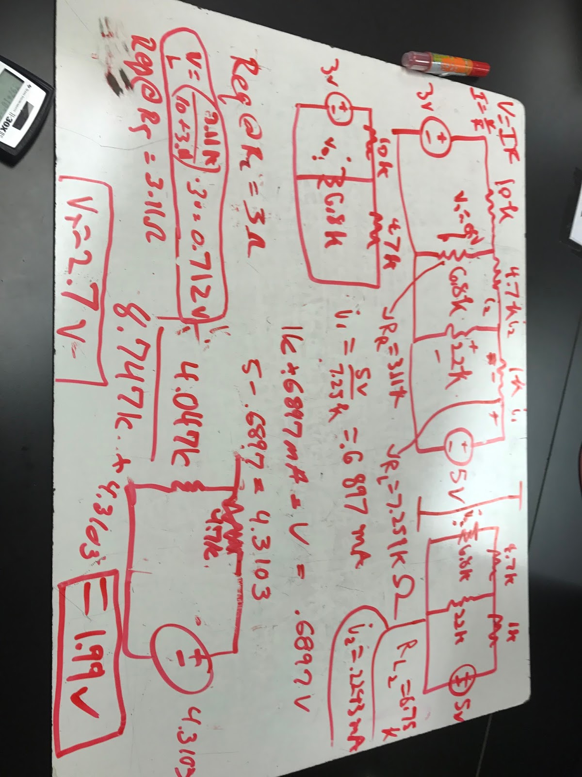
 This was the pre-lab for the superposition lab. We were very confused as to what we needed to do.

We ran out of time to build the circuit so we analyzed the circuit on every MODEL.

Lab: Mesh Analysis (March 21, 2017)

Date: 03/21/2017

Mesh Analysis 2

 In this example, we tried our hand at mesh analysis. In order to do mesh analysis, we have to do a loop that contains the current of each individual block of the circuit. Mesh analysis focuses on the voltage inside of each block of the circuit. Since we are analyzing voltage, v=ir, we can solve for the current at any given part of the circuit. (Which is what we did for this example of mesh analysis).

 We did the first example wrong, then re-did the problem getting it right in this picture.

 This in another example of mesh analysis. This type of circuit is more common than the preceding example. This is also the pre-lab for mesh analysis 2. We determined the current of circuit using matrix analysis.

 This is a diagram of the built circuit for mesh analysis 2.

 In this photo, we do mesh analysis of a transistor. In order to achieve this, we must convert the transistor from the first diagram to the second diagram. In the second diagram, all of the internal components of the transistor are shown.

 The class did not fully understand, thus, the professor had to explain on the board.

This is the built circuit for mesh analysis 2 using waveform along with a volt meter.